


In the era of Software-Defined Networking (SDN) and Cloud Networking, it is easy to abstract away the physical reality of how data moves. We often visualize networks as logical diagrams, routing tables, and API endpoints. However, at the very bottom of the OSI Model—Layer 1—lies the tangible infrastructure that makes the digital world possible: Network Cables. For the Network Engineer, System Administrator, or DevOps professional, understanding cabling is not just about plugging in a wire; it is about understanding signal integrity, bandwidth capacity, latency, and the physical limitations of data transmission.
While a user might simply see “WiFi and cables,” a seasoned professional sees a complex matrix of attenuation, crosstalk, electromagnetic interference (EMI), and maximum transmission units (MTU). The quality of the physical medium dictates the stability of the TCP/IP stack running on top of it. A single bad crimp or a fiber bend radius violation can manifest as packet loss, jitter, or inexplicable application timeouts that no amount of code optimization can fix. This article explores the technical depths of network cabling, from copper to fiber, and demonstrates how to use modern Network Automation and programming tools to diagnose physical layer issues.
The Copper Standard: Twisted Pair and Ethernet Standards
Twisted pair cabling remains the ubiquitous standard for Local Area Networks (LANs). The evolution from Cat5 to Cat8 represents a battle against physics—specifically, the fight to reduce crosstalk and increase frequency (MHz) to support higher data rates.
Categories and Shielding
The distinction between cable categories lies primarily in the twist rate (twists per inch) and shielding. Tighter twists reduce crosstalk between pairs within the cable. Shielding protects the data from external EMI.
- Cat5e: The baseline for Gigabit Ethernet (1000BASE-T). Operates at 100 MHz. While sufficient for basic home use, it is susceptible to crosstalk in high-density environments.
- Cat6: Operates at 250 MHz. Includes a physical separator (spline) between pairs to reduce crosstalk. Supports 10Gbps over short distances (up to 55 meters).
- Cat6a (Augmented): Operates at 500 MHz. Supports 10Gbps up to the full 100 meters. This is the standard for modern enterprise Network Architecture.
- Cat8: Operates at 2000 MHz (2 GHz). Heavily shielded. Designed for data centers to support 25Gbps and 40Gbps over short distances (30 meters).
When designing a network, calculating the theoretical transfer time based on cable throughput is essential for setting Service Level Agreements (SLAs). Below is a Python script that helps network architects estimate transfer times across different cable standards, aiding in capacity planning.
import math

def calculate_transfer_time(file_size_gb, bandwidth_gbps, efficiency=0.9):
    """
    Calculates estimated transfer time considering protocol overhead.

    Args:
        file_size_gb (float): Size of the file in Gigabytes
        bandwidth_gbps (float): Network speed in Gigabits per second
        efficiency (float): Network efficiency factor (TCP overhead, headers, etc.)

    Returns:
        float: Time in seconds
    """
    # Convert file size to Gigabits (1 Byte = 8 bits)
    file_size_bits = file_size_gb * 8

    # Effective bandwidth
    effective_bandwidth = bandwidth_gbps * efficiency

    time_seconds = file_size_bits / effective_bandwidth
    return time_seconds

# Scenario: Backing up a 500GB Virtual Machine image
file_size = 500

standards = {
    "Cat5e (1 Gbps)": 1.0,
    "Cat6a (10 Gbps)": 10.0,
    "Cat8 (40 Gbps)": 40.0
}

print(f"Transfer Time Estimates for {file_size} GB Data Migration:\n")
for cable, speed in standards.items():
    seconds = calculate_transfer_time(file_size, speed)
    minutes = seconds / 60
    print(f"Standard: {cable}")
    print(f"Time: {seconds:.2f} seconds ({minutes:.2f} minutes)")
    print("-" * 30)
Fiber Optics: Light, Refraction, and Distance
While copper dominates the access layer, fiber optics rule the backbone and long-haul connections. Fiber uses light pulses to transmit data, making it immune to electromagnetic interference—a critical feature for industrial environments or runs parallel to high-voltage power lines.
Single-mode vs. Multi-mode
Understanding the difference between Single-mode Fiber (SMF) and Multi-mode Fiber (MMF) is vital for Network Design and budgeting.
- Multi-mode (OM3, OM4, OM5): Uses a wider core (50 microns). Light bounces off the core walls (modal dispersion). Used for shorter distances (inside data centers or buildings) typically driven by LED or VCSEL sources. It is cheaper to implement but has distance limitations due to signal attenuation and dispersion.
- Single-mode (OS2): Uses a tiny core (9 microns). Light travels straight down the center with minimal reflection. Driven by lasers. Capable of spanning kilometers (Campus LANs, WANs, ISP backbones).
In modern Data Center environments, managing thousands of fiber connections requires rigorous monitoring. A dirty connector or a damaged cable often results in interface errors. We can use Python with the netmiko library to automate the detection of these physical layer issues on network devices like Cisco switches.
from netmiko import ConnectHandler
import json

def check_interface_errors(device_params):
    """
    Connects to a network device and checks for physical layer errors
    (CRC, Input Errors) which indicate cable issues.
    """
    try:
        connection = ConnectHandler(**device_params)
        print(f"Connected to {device_params['host']}")

        # Send command to get interface statistics
        # Note: 'show interfaces' output parsing varies by vendor
        output = connection.send_command("show interfaces | include line protocol|CRC|input errors")

        print("\n--- Physical Layer Health Check ---")
        lines = output.split('\n')

        current_interface = ""
        issues_found = False

        for line in lines:
            if "line protocol" in line:
                current_interface = line.split()[0]

            if "CRC" in line or "input errors" in line:
                # Simple parsing logic for demonstration
                parts = line.split(',')
                for part in parts:
                    if "CRC" in part:
                        crc_count = int(part.strip().split()[0])
                        if crc_count > 0:
                            print(f"[ALERT] {current_interface}: {crc_count} CRC Errors detected. Check Cable!")
                            issues_found = True
                    if "input error" in part:
                        err_count = int(part.strip().split()[0])
                        if err_count > 0:
                            print(f"[ALERT] {current_interface}: {err_count} Input Errors. Possible Duplex Mismatch or Bad Cable.")
                            issues_found = True

        if not issues_found:
            print("No significant physical layer errors detected.")

        connection.disconnect()

    except Exception as e:
        print(f"Connection failed: {e}")

# Example Device (Replace with actual credentials)
cisco_switch = {
    'device_type': 'cisco_ios',
    'host': '192.168.1.10',
    'username': 'admin',
    'password': 'secure_password',
}

# Uncomment to run in a real environment
# check_interface_errors(cisco_switch)
Advanced Diagnostics: From Layer 1 to Layer 7
Network troubleshooting often follows the “bottom-up” approach. If the cable is faulty, the HTTP Protocol will fail, DNS Protocol lookups will time out, and VPN connections will drop. However, physical faults can be subtle. A cable might negotiate at 1Gbps but drop packets under load due to near-end crosstalk (NEXT) or impedance mismatch.
Bandwidth vs. Throughput
Bandwidth is the theoretical capacity of the cable (e.g., 1 Gbps). Throughput is the actual amount of data successfully moved. A damaged cable often results in high retransmission rates in TCP/IP, lowering effective throughput. Tools like iPerf3 are standard for verifying if a cable run can actually sustain its rated speed.
Below is a shell script example that automates iPerf3 testing, a common task for a Network Engineer or System Administrator verifying new cabling installations.
#!/bin/bash

# Network Cable Throughput Validator
# Requires iperf3 installed on both ends
# Usage: ./cable_test.sh <server_ip>

SERVER_IP=$1
DURATION=10
PARALLEL_STREAMS=4

if [ -z "$SERVER_IP" ]; then
    echo "Usage: $0 <server_ip>"
    exit 1
fi

echo "------------------------------------------------"
echo "Starting Cable Integrity Test to $SERVER_IP"
echo "Testing TCP Throughput and Jitter..."
echo "------------------------------------------------"

# Run iPerf3 client
# -c: client mode
# -t: time in seconds
# -P: parallel streams (saturates the link to test cable stress)
# -J: Output in JSON for parsing (optional)

iperf3 -c $SERVER_IP -t $DURATION -P $PARALLEL_STREAMS > cable_test_results.txt

# Extract Bandwidth
BITRATE=$(grep "SUM" cable_test_results.txt | tail -n 1 | awk '{print $6, $7}')
RETRANSMITS=$(grep "sender" cable_test_results.txt | tail -n 1 | awk '{print $9}')

echo "Test Complete."
echo "Aggregated Throughput: $BITRATE"
echo "TCP Retransmissions: $RETRANSMITS"

if [ "$RETRANSMITS" -gt 10 ]; then
    echo "[WARNING] High retransmission count detected."
    echo "Possible causes: Damaged cable, EMI interference, or bad termination."
else
    echo "[SUCCESS] Cable run appears healthy."
fi
Protocol Analysis and Cabling
When physical tools (like Fluke testers) are unavailable, protocol analysis via Wireshark or tcpdump becomes the primary diagnostic tool. Physical layer issues often manifest in the Transport Layer (Layer 4) or Network Layer (Layer 3).
Common indicators of cabling faults in packet captures include:
- TCP Retransmissions: The packet was corrupted on the wire (CRC error) and dropped by the receiver, forcing the sender to try again.
- Duplicate ACKs: Indicative of packet loss.
- Fragmented Packets: While sometimes an MTU configuration issue, inconsistent fragmentation can indicate intermittent signal loss.
For modern Network Monitoring, we can use Python’s scapy library to perform a custom latency and jitter test. Unlike a standard ping, this can be customized to send specific packet sizes to test MTU limits on the wire.

from scapy.all import *
import time
import statistics

def cable_latency_test(target_ip, count=20, payload_size=1000):
    """
    Sends ICMP packets with a specific payload size to test cable stability.
    Large payloads on bad cables often result in drops.
    """
    print(f"Testing connectivity to {target_ip} with {payload_size} bytes payload...")

    rtt_list = []
    dropped = 0

    # Create a payload of specified size (padding)
    data = "X" * payload_size

    for i in range(count):
        packet = IP(dst=target_ip)/ICMP()/Raw(load=data)

        start_time = time.time()
        reply = sr1(packet, timeout=2, verbose=0)
        end_time = time.time()

        if reply:
            rtt = (end_time - start_time) * 1000 # ms
            rtt_list.append(rtt)
            print(f"Seq={i} | RTT={rtt:.2f}ms")
        else:
            print(f"Seq={i} | Request Timed Out")
            dropped += 1

    # Analysis
    if rtt_list:
        avg_rtt = statistics.mean(rtt_list)
        jitter = statistics.stdev(rtt_list) if len(rtt_list) > 1 else 0
        loss_pct = (dropped / count) * 100

        print("\n--- Cable Stability Report ---")
        print(f"Packet Loss: {loss_pct}%")
        print(f"Average Latency: {avg_rtt:.2f}ms")
        print(f"Jitter: {jitter:.2f}ms")

        if loss_pct > 0 or jitter > 10:
            print("[FAIL] Unstable connection. Inspect physical layer.")
        else:
            print("[PASS] Connection stable.")
    else:
        print("[CRITICAL] No connectivity. Check if cable is plugged in.")

# Note: Requires root/admin privileges to send ICMP
# cable_latency_test("8.8.8.8")
Best Practices for Network Infrastructure
Whether you are setting up a home lab, a Digital Nomad workspace, or an enterprise data center, adhering to cabling best practices ensures longevity and performance. The role of the Network Engineer is to ensure these standards are met to support advanced technologies like Edge Computing and Microservices.
Cable Management and Environment
Bend Radius: Every cable type has a minimum bend radius. Exceeding this (bending the cable too sharply) causes micro-cracks in glass fiber or alters the twist geometry in copper, leading to attenuation and signal loss.
EMI Avoidance: Never run unshielded copper network cables parallel to power cables. The electromagnetic field from the power line induces noise into the data cable. If they must cross, they should do so at a 90-degree angle.
Labeling and Documentation
In the world of DevOps Networking and Network Automation, “Infrastructure as Code” is a popular concept. However, physical infrastructure must be documented as well. Every cable should be labeled at both ends. An undocumented cable is a liability. Maintaining a “Source of Truth” (like NetBox) for physical connections is as critical as managing your API Security keys.
Power over Ethernet (PoE) Considerations
With the rise of IoT and Wireless Networking access points, PoE is standard. However, PoE generates heat within the cable bundles. When running high-power PoE (like 802.3bt Type 4), using Cat6a is recommended over Cat5e because the thicker gauge copper handles heat dissipation better, preventing signal degradation.
Conclusion
Network cables are the unsung heroes of the digital age. While the industry buzzes about Serverless architecture, GraphQL APIs, and Service Mesh implementations, none of these technologies function without the physical layer. For the Network Admin, the view of the network is not just abstract connections; it is a tangible reality of electrons and photons moving through copper and glass.
By mastering the physical layer—understanding the difference between Cat6 and Cat6a, recognizing the symptoms of dirty fiber, and utilizing Python and network tools to automate diagnostics—you elevate your skill set from a standard user to a true Network Engineer. The next time you troubleshoot a slow API response or a dropped VPN connection, remember to look down the stack. The problem might not be in the code; it might be in the cable.