The Backbone of Connectivity: A Comprehensive Guide to Network Cables and Infrastructure Management

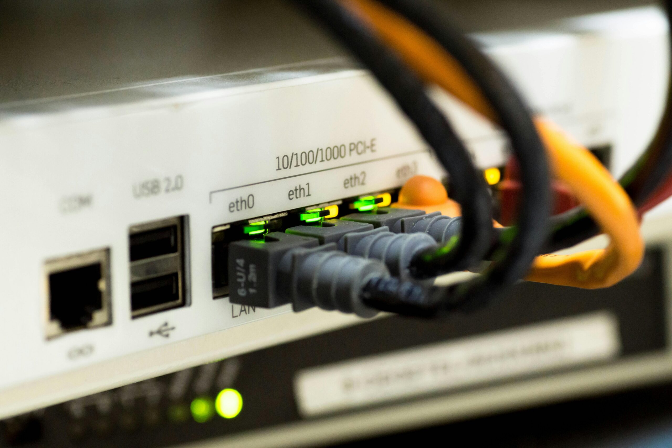
Introduction to the Physical Layer

In the era of Cloud Networking and serverless architectures, it is easy to forget that the internet is, at its core, a physical entity. While Software-Defined Networking (SDN) and Network Virtualization abstract the complexities of hardware, data transmission ultimately relies on the physical medium—Layer 1 of the OSI Model. Network cables serve as the fundamental arteries of global communication, facilitating everything from local LAN file transfers to massive Data Center Interconnect (DCI) flows that power the modern web.

For the Network Engineer and System Administration professionals, understanding the nuances of cabling is not merely about plugging in wires; it is about understanding bandwidth constraints, latency implications, and signal integrity. Whether you are designing a spine-leaf architecture for a data center or setting up a robust home office for Remote Work as a Digital Nomad, the choice of medium—Copper vs. Fiber, DAC vs. AOC—dictates the performance ceiling of your network.

This article delves deep into the technical specifications of network cabling, the protocols that run over them (Ethernet, TCP/IP), and how modern DevOps Networking practices allow us to manage, monitor, and troubleshoot the physical layer using code. We will explore how to automate interface diagnostics, calculate optical budgets, and ensure your physical infrastructure can handle the explosive growth of data traffic.

Section 1: Core Concepts of Network Cabling and Standards

The Evolution of Ethernet and Copper Cabling

Ethernet standards have evolved rapidly to keep pace with the demands of HTTP Protocol traffic and heavy media streaming. Twisted pair copper cabling remains the standard for access layers due to its cost-effectiveness and durability. The twisted pair design minimizes electromagnetic interference (EMI) and crosstalk, which is crucial for maintaining signal integrity.

Common categories include:

• Cat5e: Supports 1 Gbps up to 100 meters. Now considered legacy but still prevalent.
• Cat6: Supports 10 Gbps up to 55 meters. The standard for modern office deployments.
• Cat6a: Supports 10 Gbps up to 100 meters with better shielding (STP/FTP) against alien crosstalk.
• Cat8: Supports 25/40 Gbps over short distances (30 meters), primarily for data center switch-to-server connections.

Fiber Optics: The Speed of Light

For long-distance transmission and high-bandwidth Data Center Interconnects, fiber optics are mandatory. Unlike copper, which uses electrical signals, fiber uses pulses of light, making it immune to EMI and capable of significantly lower Latency.

Single-Mode Fiber (SMF): Uses a tiny core (9 microns) to transmit a single ray of light. It eliminates modal dispersion, allowing signals to travel dozens of kilometers. This is essential for WAN links and connecting geographically separated availability zones.

Multi-Mode Fiber (MMF): Uses a wider core (50 or 62.5 microns). It is cheaper to manufacture and uses lower-cost light sources (LED/VCSEL) but is limited by modal dispersion to shorter distances (usually under 400 meters). It is the backbone of intra-building backbones.

Programmatic Cable Management

In modern Network Architecture, documentation is code. Managing a complex inventory of cables, transceivers, and patch panels requires structured data. Below is a Python example using object-oriented principles to model cable constraints, a concept useful for Network Automation tools.

class NetworkCable:
    def __init__(self, cable_type, category, max_length_meters):
        self.cable_type = cable_type  # e.g., 'Copper', 'Fiber'
        self.category = category      # e.g., 'Cat6a', 'OM4'
        self.max_length = max_length_meters

    def validate_link(self, distance_meters, required_bandwidth_gbps):
        """
        Validates if the cable can support the requested distance and speed.
        """
        if distance_meters > self.max_length:
            return False, f"Distance {distance_meters}m exceeds limit for {self.category}"
        
        # Simplified bandwidth capability check
        capabilities = {
            'Cat5e': 1,
            'Cat6': 10 if distance_meters <= 55 else 1,
            'Cat6a': 10,
            'OM4': 100 if distance_meters <= 150 else 10,
            'OS2': 400 # Single mode theoretical high limit
        }
        
        limit = capabilities.get(self.category, 0)
        if required_bandwidth_gbps > limit:
            return False, f"Bandwidth {required_bandwidth_gbps}Gbps exceeds limit for {self.category}"
            
        return True, "Link Valid"

# Example Usage
dc_link = NetworkCable('Fiber', 'OM4', 400)
is_valid, message = dc_link.validate_link(100, 40) # 100 meters at 40Gbps

print(f"Cable Check: {message}")

Section 2: Implementation and Data Center Interconnects

Direct Attach and Active Optical Cables

In high-performance computing and dense switching environments, standard patch cables are often replaced by Direct Attach Copper (DAC) and Active Optical Cables (AOC). These are pre-terminated cable assemblies used to connect switches to routers or servers within the same rack or adjacent racks.

DACs are passive copper cables with transceivers attached. They offer the lowest latency and power consumption but are limited to very short distances (3-7 meters). They are ideal for Top-of-Rack (ToR) switching.

AOCs are fiber cables with embedded electronics that convert electrical signals to optical and back. They reach further (up to 100 meters) and are lighter and thinner than DACs, improving airflow management in racks—a critical factor in Network Design.

Detecting Physical Layer Errors via Automation

A bad cable often manifests as intermittent packet loss, CRC errors, or “flapping” interfaces. In a manual workflow, a Network Engineer might stare at CLI output. In a DevOps Networking workflow, we use Network Libraries like Netmiko or Paramiko to automate this detection. This is vital for maintaining high Network Performance.

The following script demonstrates how to connect to a network device, retrieve interface statistics, and identify ports that may have faulty cabling based on CRC error counters.

from netmiko import ConnectHandler
import json

def check_physical_errors(device_params):
    """
    Connects to a switch and checks for CRC errors indicating cable faults.
    """
    try:
        net_connect = ConnectHandler(**device_params)
        
        # Command varies by vendor; this is a generic Cisco/Arista example
        # In a real scenario, use structured output (TextFSM) or REST API
        output = net_connect.send_command("show interfaces | include CRC")
        
        lines = output.split('\n')
        error_ports = []
        
        for line in lines:
            if "CRC" in line:
                # Simple parsing logic
                parts = line.split()
                crc_count = int(parts[0]) # Assuming count is first for this example context
                if crc_count > 0:
                    error_ports.append(line)
        
        net_connect.disconnect()
        return error_ports

    except Exception as e:
        return [f"Connection failed: {str(e)}"]

# Mock device parameters
switch = {
    'device_type': 'cisco_ios',
    'host': '192.168.1.10',
    'username': 'admin',
    'password': 'secure_password',
}

# In a production environment, this would integrate with monitoring tools
# print(check_physical_errors(switch))

Optical Power Budgets

When dealing with fiber, light attenuates (losses intensity) as it travels through the cable, splices, and connectors. If the light is too weak, the receiver cannot interpret the data (packet loss). If it is too strong, it can burn out the receiver. Calculating the “Optical Loss Budget” is a critical skill in Network Engineering.

Formula: Link Loss = (Cable Length * Attenuation per km) + (Number of Splices * Splice Loss) + (Number of Connectors * Connector Loss)

Section 3: Advanced Techniques and Diagnostics

Packet Analysis and Physical Layer Troubleshooting

Sometimes, the interface shows “UP,” but applications are slow. This requires Packet Analysis using tools like Wireshark. At the TCP/IP level, a bad cable often results in TCP Retransmissions or fragmented packets. While Wireshark analyzes the bits, the root cause is often the atoms—the copper or glass.

Using Python’s scapy library, we can analyze PCAP files programmatically to correlate retransmission spikes with specific timeframes, helping to isolate physical layer degradation that might occur only during peak heat or load.

from scapy.all import rdpcap, TCP

def analyze_retransmissions(pcap_file):
    """
    Analyzes a PCAP file to count TCP retransmissions.
    High retransmission rates often correlate with physical layer packet loss.
    """
    packets = rdpcap(pcap_file)
    retransmissions = 0
    total_tcp = 0
    
    # Dictionary to track sequence numbers per flow
    flows = {} 

    for pkt in packets:
        if TCP in pkt:
            total_tcp += 1
            # Define flow by src/dst IP and Port
            flow_id = (pkt['IP'].src, pkt['TCP'].sport, pkt['IP'].dst, pkt['TCP'].dport)
            seq = pkt['TCP'].seq
            
            if flow_id in flows:
                if seq in flows[flow_id]:
                    retransmissions += 1
                else:
                    flows[flow_id].add(seq)
            else:
                flows[flow_id] = {seq}

    loss_rate = (retransmissions / total_tcp) * 100 if total_tcp > 0 else 0
    
    return {
        "total_tcp_packets": total_tcp,
        "retransmissions": retransmissions,
        "retransmission_rate_percent": round(loss_rate, 2)
    }

# usage: results = analyze_retransmissions('capture.pcap')

Infrastructure as Code (IaC) for Cabling

In advanced Cloud Networking and Service Mesh environments, the physical underlay is often documented using Infrastructure as Code principles. Tools like NetBox serve as a “Source of Truth.” Using REST APIs, we can enforce cabling standards. For instance, ensuring that a 100Gbps interface is only documented as connected to a valid SMF or OM4 cable type.

Below is an example of how one might validate cable connections against a defined standard using a JSON structure, simulating an API response from a documentation system.

// Example JSON structure representing a connection in a DC
const connectionData = {
    "source_device": "leaf-switch-01",
    "source_port": "Ethernet1/1",
    "dest_device": "compute-node-05",
    "dest_port": "eth0",
    "cable_type": "DAC",
    "length_meters": 3,
    "speed_gbps": 25
};

function validateCablingStandard(connection) {
    // Rule: DAC cables should not exceed 5 meters for 25Gbps to ensure integrity
    const MAX_DAC_LENGTH = 5;
    
    if (connection.cable_type === "DAC") {
        if (connection.length_meters > MAX_DAC_LENGTH) {
            return `VIOLATION: DAC cable too long (${connection.length_meters}m) for reliable 25G transmission.`;
        }
    }
    
    // Rule: High speed uplinks usually require Fiber
    if (connection.speed_gbps >= 100 && connection.cable_type === "Cat6a") {
        return "VIOLATION: Cannot use Copper Cat6a for 100Gbps links.";
    }

    return "COMPLIANT: Cabling standard met.";
}

console.log(validateCablingStandard(connectionData));

Section 4: Best Practices and Future Trends

Cable Management and Airflow

Proper cable management is not just about aesthetics; it is a functional requirement for Network Security and hardware longevity. In dense server racks, “spaghetti cabling” blocks exhaust fans, causing servers to overheat. This thermal throttling reduces CPU performance and can lead to hardware failure. Velcro ties should always be used over zip ties to prevent crushing the internal geometry of twisted pairs or micro-bending fiber optics, which causes light leakage (attenuation).

Security at Layer 1

Network Security often focuses on Firewalls and HTTPS Protocol encryption, but physical security is paramount. Unused ports should be administratively down. In high-security environments, fiber taps can intercept data without breaking the link. Technologies like MACsec (802.1AE) provide encryption at Layer 2 to mitigate physical tapping risks, ensuring that even if the cable is compromised, the data remains unreadable.

Future-Proofing: 400G and Beyond

As we move toward 400G and 800G standards to support Edge Computing and AI workloads, the physics of cabling becomes even more critical. We are seeing a shift toward parallel optics (MPO connectors) where one cable contains 12, 24, or even 32 strands of fiber. For the “Tech Travel” enthusiast or Digital Nomad, this infrastructure evolution eventually translates to faster 5G/6G backhauls, enabling seamless Remote Work from anywhere in the world.

Labeling and Documentation

Every cable must be labeled at both ends. The ANSI/TIA-606-B standard provides guidelines for administration. However, in the age of Network Automation, digital documentation in a tool like NetBox or Nautobot is essential. If the physical reality deviates from the digital documentation, automation scripts will fail, leading to extended downtime during Network Troubleshooting.

Conclusion

Network cables are the unsung heroes of the digital age. From the subsea fiber optics carrying DNS Protocol queries across oceans to the short DACs connecting microservices in a Kubernetes cluster, the physical layer dictates the reliability and speed of our connected world. For the modern Network Engineer, understanding the physics of these cables and mastering the Network Tools to manage them programmatically is no longer optional.

By integrating physical layer management with software concepts—using Python for diagnostics, JSON for documentation, and APIs for monitoring—we bridge the gap between hardware and code. As bandwidth demands continue to skyrocket with the adoption of 4K streaming, VR, and massive AI models, the ability to tame the “wildest” part of the network through disciplined cabling standards and automation will separate robust enterprise networks from fragile ones.

Whether you are debugging a home lab or architecting a global ISP backbone, remember: the cloud is just someone else’s computer, and that computer is connected by a cable. Treat Layer 1 with the respect it deserves, and your upper-layer protocols will thank you.